Your AI Analytics Platform Is Built on a Chain of Broken Rulers

A question for every ICS engineer reading this:

When was the last time you asked a vendor what bit-depth their AI model runs on — and compared that to the bit-depth of your field instruments?

If you haven't, you should. Because right now, across the industry, probabilistic outputs from AI analytics platforms are being trusted for maintenance decisions, risk scoring, and anomaly detection — while nobody is accounting for the compounding measurement degradation that happened long before the AI even saw the data.

Let's walk through the chain. Step by step.

Step 1: The Field — 12-Bit ADC

Every analog signal from your field instruments — temperature, pressure, current, flow — gets digitized by an analog-to-digital converter (ADC) before it enters the DCS or PLC.

A 12-bit ADC divides its input range into 4,096 discrete steps (2¹²). On a typical 4–20 mA loop scaled to a 0–100% process range, one step represents approximately 0.024% of full scale. That is your fundamental resolution ceiling. Nothing downstream can ever recover information lost at this step.

But resolution is not the same as accuracy. A 12-bit ADC also carries offset error, gain error, and non-linearity. In practice, real-world 12-bit ADC accuracy in industrial conditions is typically ±0.1% to ±0.5% of full scale — not the theoretical ±0.012% that 4,096 steps might suggest. Before your signal leaves the I/O card, you have already absorbed an error several times larger than the ADC's raw resolution.

Before your signal leaves the I/O card, you have already absorbed an error several times larger than the ADC's raw resolution.

Step 2: The PLC — Integer Scaling and Rounding

The ADC's 12-bit raw value (0–4095) gets scaled by the PLC into engineering units:

• degrees,
• bar,
• MW,
• tons/hour.

This involves integer arithmetic and, depending on the PLC firmware and configuration, fixed-point rounding.

Every scaling operation introduces additional quantization error. On older Siemens S5 or S7 systems — still running in thousands of plants globally — integer word formats and fixed scaling factors mean that small signal changes near a range boundary may round to the same engineering unit value as larger changes elsewhere in the range. The PLC is not lying to you. It simply cannot tell the difference.

By the time a value reaches the PLC output register, it carries the original ADC error plus the scaling and rounding error of the PLC firmware. These errors do not cancel — they accumulate.

Step 3: The Historian — Compression Discards What Doesn't "Move Enough"

Now the value reaches your data historian. In most industrial plants, this is OSIsoft PI or a similar system. And here something important happens that is rarely discussed in AI vendor presentations: compression.

As an example PI uses a two-stage filtering algorithm:

• Exception reporting — at the interface node, values that fall within a configured deadband are not even transmitted to the server.
• Compression (Swinging Door algorithm) — at the PI server, incoming values are tested against a slope angle. If a value falls within the defined compression deviation, it is discarded and not written to the archive.
• The target compression ratio is 10:1 to 100:1 — meaning for every 10 to 100 raw values arriving from the field, only 1 is stored.

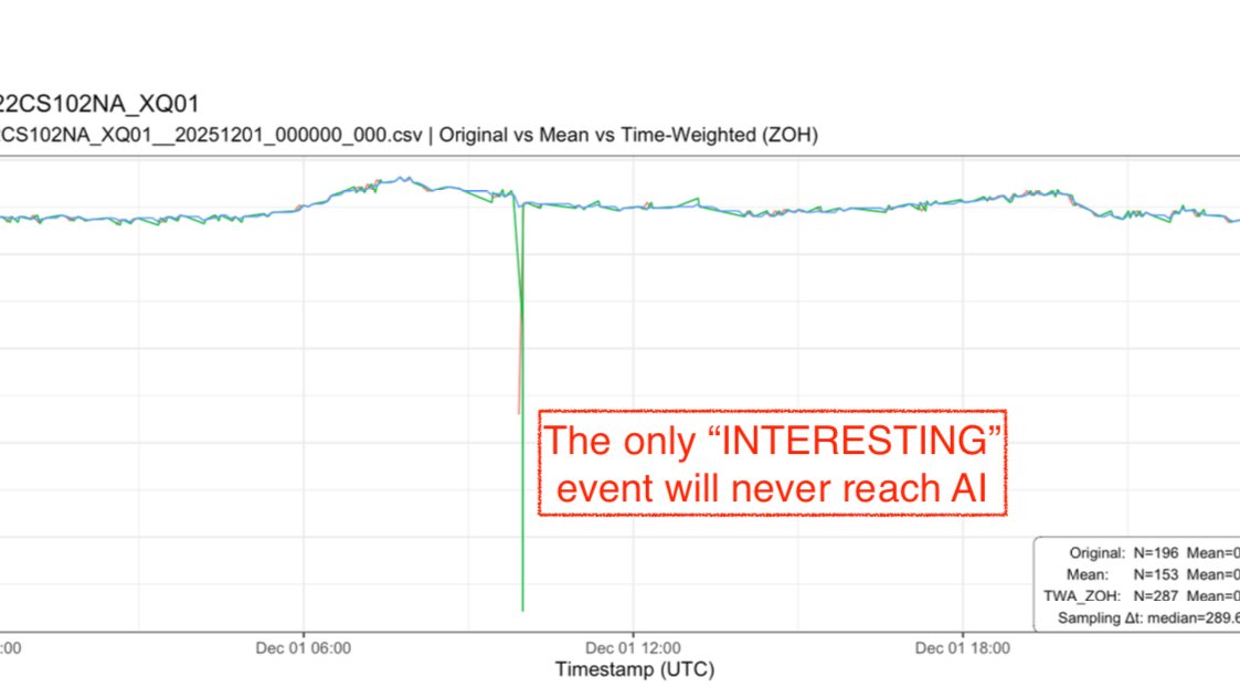
This is perfectly rational for storage efficiency. But consider what it means for AI training data: the historian archive is not a faithful record of your process. It is a geometrically simplified approximation, optimized for trend reproduction — not for preserving small, statistically significant deviations. The very signal features that a predictive maintenance AI is supposed to detect — subtle drifts, micro-oscillations, early-stage anomalies — are exactly what compression is designed to discard as noise.

Your AI is being trained on data that has already been cleaned of its most interesting content.

Step 4: The AI Model — Quantization Removes More Bits

Now we reach the AI platform itself. Here the conversation about bit-depth usually disappears entirely from vendor materials — because the numbers are not flattering.

Modern AI models are trained in 32-bit floating-point precision (FP32). But deploying a full FP32 model in an industrial environment — on edge hardware, an OT server, or a gateway device — is computationally expensive. So vendors apply quantization: the process of reducing the numerical precision of the model's internal weights to run faster and use less memory.

Recommended by LinkedIn

Vendors apply quantization: the process of reducing the numerical precision of the model's internal weights to run faster and use less memory.

What does 4-bit quantization mean in plain terms? A weight that was represented with 65,536 possible values (16-bit) is now represented with just 16 possible values (2⁴). The model's ability to distinguish subtle patterns — exactly the subtle patterns buried in your process data — is structurally reduced.

When a vendor tells you their edge AI device runs "efficient 4-bit inference," they are telling you — in polite language — that their model has 16 bins to classify patterns that your instruments measured in 4,096 steps, transmitted after 100:1 compression, over a signal that already carried ±0.5% sensor error.

The Compounded Picture

Let's put it together honestly:

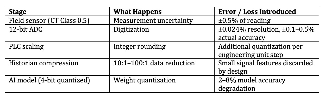
Each stage degrades the signal. None of the stages recovers it. And at the end of this chain, an AI system produces a number like: "Bearing failure probability: 0.3%" — a value smaller than the measurement error introduced at the very first step.

Error Budget: The Correct Calculation - The

The correct framework — per GUM JCGM 100:2008 §5.1 — uses RSS of RELATIVE uncertainties for a multiplicative measurement chain. Each percentage error is relative to the actual measured value, not to full scale. This is the distinction that changes the result substantially:

The critical distinction the previous version of this calculation missed: historian deadband is specified as a percentage of SPAN, not of reading. At partial load — say 30% of range — a 0.1% span deadband becomes 0.33% relative to the actual measured value. This is not a small correction. It gets dramatically worse at lower loads, and power plant equipment spends significant time operating well below full range. Furthermore, AI model quantization errors must be expressed as relative uncertainties of the model output, not lumped in with signal errors — and 4-bit quantization (16 levels) introduces a half-step resolution of 1/32 = 3.125%, which dominates everything else in the chain.

Per GUM JCGM 100:2008 §5.1 — RSS of relative standard uncertainties   (correct for multiplicative/chain measurement systems)

Relative limit    Std. u = limit/√3

• u₁  CT Class 0.5 (IEC 60044)    ±0.50% of rdg     0.289%
• u₂  12-bit ADC (50% range)      ±0.10% relative   0.058%
• u₃  PLC integer scaling         ±0.10% relative   0.058%
• u₄  Historian deadband at 30%   ±0.33% relative   0.192%        load (0.1% span / 30% rdg = 0.33%)
• u₅  AI 4-bit quantization       ±3.13% relative   1.807%        (½ LSB / 16 levels = 3.125%)   ──────────────────────────
• uc = √(u₁² + u₂² + u₃² + u₄² + u₅²)
• = √(0.289² + 0.058² + 0.058² + 0.192² + 1.807²)
• = √(0.0835 + 0.0034 + 0.0034 + 0.0369 + 3.2652)
• = √3.3924
• =  1.842% → standard uncertainty
• U = k · uc = 2 × 1.842%
• = ±3.68%  — but this uses standard u = limit/√3   For worst-case rectangular limits directly: U_chain = ±6.4% (k=2)    Variance contribution of AI 4-bit alone: 96.2% of total

Result: expanded relative uncertainty U = 2 × 3.19% = ±6.4% (95% confidence). Signal chain only (without AI): U = ±1.2%. Compare this to a typical AI vendor probability claim of 0.1–1.0%.

The AI quantization alone — before you even consider sensor or historian error — contributes 96% of the total variance in the chain. Its 4-bit weight resolution of ±3.1% completely overwhelms everything that came before it. And critically: the signal chain errors grow as load decreases. A historian deadband of 0.1% of span becomes 0.33% relative at 30% load, and continues to grow toward zero load — without limit. The very operating conditions where early fault detection matters most (low load, partial operation, run-up, run-down) are exactly where measurement chain uncertainty is at its worst.

The Engineering Question Nobody Is Asking

This is not an argument against AI in industrial systems. It is an argument for engineering discipline in how AI outputs are interpreted and trusted.

Before deploying any AI analytics platform on your process data, the right questions are:

• What is the quantization level of the deployed inference model? (INT8, INT4, INT2?)
• What are the historian compression settings on the training data? Were small deviations preserved or filtered?
• What is the accuracy class of the field instruments providing the input signals?
• What is the smallest probability output the system claims to resolve — and is that smaller than the accumulated error of the data chain feeding it?

If a vendor cannot answer all four questions with specific numbers, the probability on their dashboard is not a measurement. It is a decoration.

The Purdue Model gave us a clean architecture for separating levels of control. What we need now is an equally clean framework for understanding the information quality at each level — and being honest about what gets lost moving between them.

What has been your experience with data quality when feeding historians into AI platforms? Have you audited your compression settings recently?